Continuous Charge Distribution and Gauss's Law

When you first study electrostatics, the world seems beautifully simple. You are introduced to “point charges”—infinitely small, perfectly round mathematical dots floating in a vacuum. You learn Coulomb’s Law, you calculate the force between two of these magical dots, and everything makes sense.

But then, reality hits.

In the real world, electric charge doesn’t exist as isolated mathematical points. It exists on the surface of your phone screen, along the length of copper wires, and distributed throughout the volume of a thundercloud. When trillions of electrons gather on a physical object, it is impossible to calculate the electric field by adding up the force of each individual electron.

To tackle this issue, we need to use the concept of Continuous Charge Distribution. It solves our problem very easily and beautifully. Let’s take a deeper look at it.

Key Takeaways

• The Big Three Densities: Charge can be distributed linearly along a wire ($\lambda$), across a 2D surface ($\sigma$), or throughout a 3D volume ($\rho$).
• Area is a Vector: In advanced physics, the area of a surface has a direction, always pointing perfectly perpendicular (normal) to the surface itself.
• Electric Flux: This is a measure of how many electric field lines “flow” through a given area.
• Gauss’s Law: A powerful theorem stating that the total electric flux out of any closed mathematical surface is directly proportional to the total electric charge enclosed within it.

---

1. The Three Types of Continuous Charge Distribution

When dealing with macroscopic objects (like a metal rod or a plastic sphere), the number of elementary charges (electrons or protons) is so incredibly large that we can treat the charge as if it is smeared out continuously over the object. Depending on the shape of the object, we categorize this distribution into three types.

Linear Charge Density ($\lambda$)

If you have a very long, incredibly thin object—like a copper wire or a carbon nanotube—the charge is distributed along a single dimension: its length.

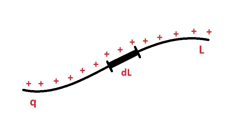
We define the Linear Charge Density (denoted by the Greek letter lambda, $\lambda$) as the amount of charge per unit length.

• Formula: $\lambda = \frac{q}{L}$ (or for infinitesimally small sections: $\lambda = \frac{dq}{dl}$)
• SI Unit: Coulomb per meter ($\text{C m}^{-1}$)
• Total Charge: If you know the linear charge density, the total charge on a wire of length $L$ is exactly $Q = \lambda L$.

Surface Charge Density ($\sigma$)

When charge spreads out over a two-dimensional area—like a sheet of graphene or the metal casing of a capacitor—we use Surface Charge Density (denoted by sigma, $\sigma$).

• Formula: $\sigma = \frac{q}{A}$ (or $\sigma = \frac{dq}{da}$)
• SI Unit: Coulomb per square meter ($\text{C m}^{-2}$)
• Total Charge: For a uniform sheet of area $A$, the total charge is $Q = \sigma A$.

Volume Charge Density ($\rho$)

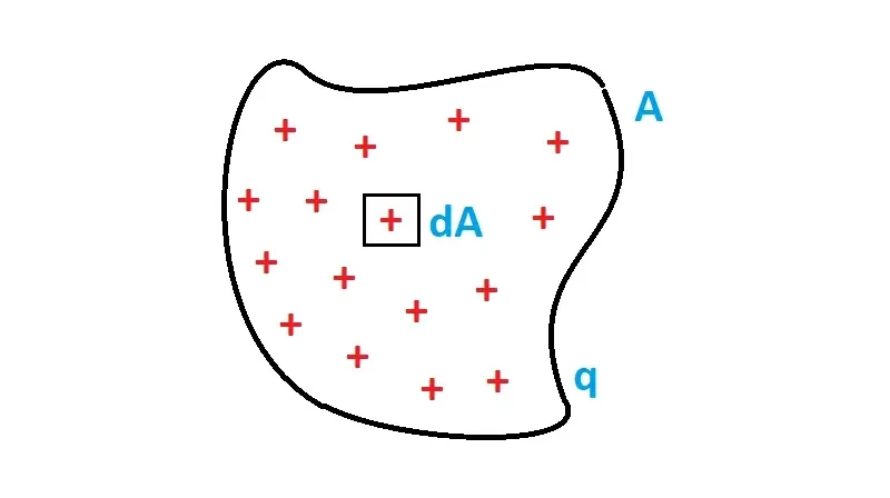
Finally, if the charge is distributed throughout the entire three-dimensional body of an object—such as a solid insulating sphere—we use Volume Charge Density (denoted by rho, $\rho$).

• Formula: $\rho = \frac{q}{V}$ (or $\rho = \frac{dq}{dv}$)
• SI Unit: Coulomb per cubic meter ($\text{C m}^{-3}$)
• Total Charge: The total charge contained in a volume $V$ is $Q = \rho V$.

---

2. The Area Vector: When Area Gets a Direction

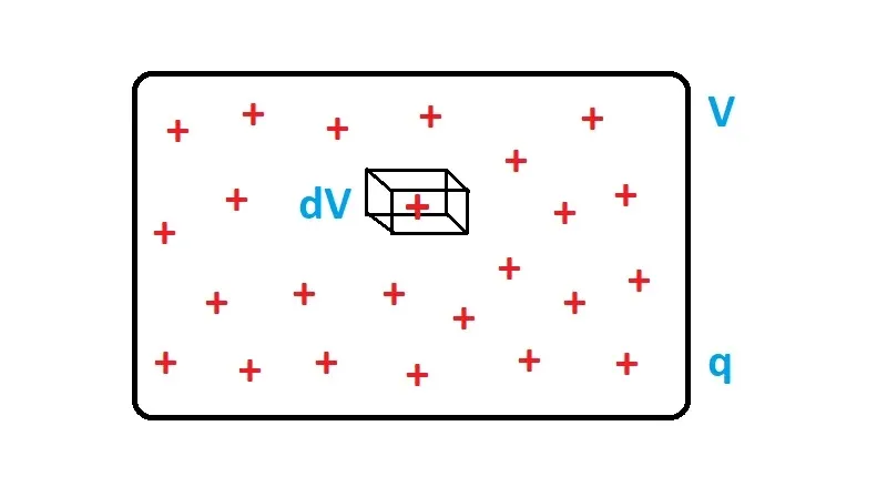
Before we can understand electric flux, we have to rethink something you learned in elementary school: Area.

In geometry, area is just a scalar number (e.g., 5 square meters). But in advanced physics, the orientation of that area matters immensely. Imagine holding a solar panel facing directly into the sun versus holding it edge-on. The physical size of the panel hasn’t changed, but its orientation dictates how much light it catches.

To account for this mathematically, we treat Area as a vector ($\vec{A}$).

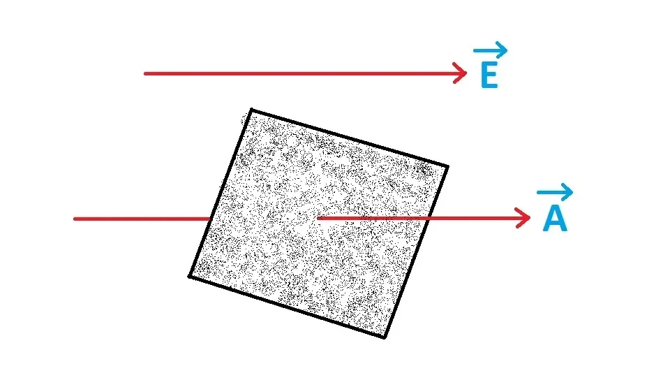
The Area Vector has a magnitude equal to the physical area of the surface, and its direction is strictly perpendicular (normal) to that surface.

$\vec{A} = A\hat{n}$

(Where $\hat{n}$ is the unit vector indicating the perpendicular direction).

Open vs. Closed Surfaces

For an open surface (like a flat sheet of paper), there are two possible perpendicular directions (up or down). By convention, we usually choose the direction that points generally along the electric field lines.

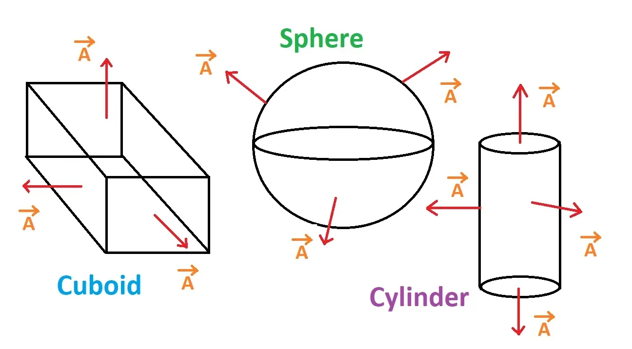
For a closed surface (like a sphere or a cube that traps a volume inside), the rule is strict: the Area Vector always points outward, away from the inside volume.

---

3. Electric Flux ($\phi$)

Now that we understand Area Vectors, we can define Electric Flux.

Electric flux is a mathematical measure of how many electric field lines pass through a given surface. Think of it like a net catching water in a river. If the net is perpendicular to the current, it catches the maximum amount of water. If you turn the net perfectly sideways, the water flows right past it, and you catch nothing.

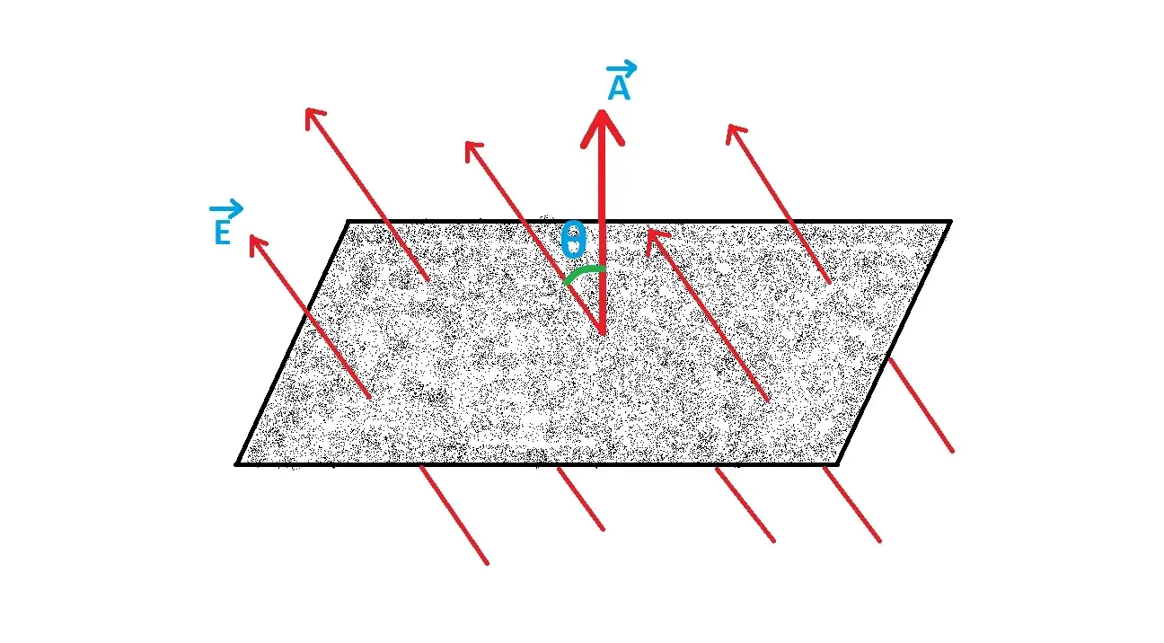
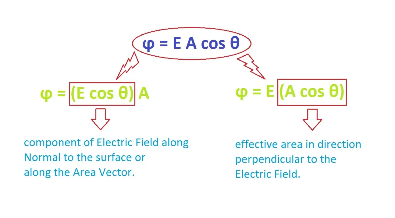
Mathematically, Electric Flux ($\phi$) is defined as the dot product of the Electric Field vector ($\vec{E}$) and the Area vector ($\vec{A}$):

$\phi = \vec{E} \cdot \vec{A}$ $\phi = E A \cos(\theta)$

Where $\theta$ is the angle between the Electric Field and the Area Vector.

• If $\theta = 0^\circ$, $\cos(0) = 1$, and flux is at its absolute maximum.
• If $\theta = 90^\circ$, $\cos(90) = 0$, and the flux is precisely zero.

Dimensional Formula: $[M L^3 T^{-3} A^{-1}]$
SI Unit: Newton-square meters per Coulomb ($\text{N m}^2 \text{C}^{-1}$) or Volt-meters ($\text{V m}$).

If the electric field is non-uniform or the surface is highly curved, we break the surface down into infinitesimally small area vectors ($d\vec{A}$) and integrate over the entire surface:

$\phi = \int \vec{E} \cdot d\vec{A}$

---

4. Gauss’s Law: The Crown Jewel of Electrostatics

In 1813, the brilliant mathematician Carl Friedrich Gauss formulated a theorem that completely revolutionized how we calculate electric fields.

Gauss’s Law states: The total electric flux passing through any closed mathematical surface (a Gaussian surface) is exactly equal to the total net electric charge enclosed by that surface, divided by the permittivity of free space ($\epsilon_0$).

Mathematically, it is expressed as:

$\oint \vec{E} \cdot d\vec{A} = \frac{Q_{\text{enc}}}{\epsilon_0}$

Where:

• $\oint$ represents a closed surface integral (the circle on the integral sign means the surface must be completely closed, like a sphere or a box, with no holes).
• $Q_{\text{enc}}$ is the net charge strictly inside the imaginary surface. Charges outside the surface contribute nothing to the total net flux!
• $\epsilon_0$ is the vacuum permittivity constant ($8.854 \times 10^{-12} \, \text{F m}^{-1}$).

Gauss’s law is incredibly powerful because it allows us to bypass horrific, complex calculus when dealing with symmetrical charge distributions. By simply drawing an imaginary “Gaussian” shape around a charged object, we can find the electric field in two lines of algebra.

---

5. Applications of Gauss’s Law

To truly appreciate the power of Gauss’s Law, let’s look at three classic derivations where it turns an impossible math problem into a trivial one.

I. Derivation of Coulomb’s Law

Imagine a single positive point charge ($Q$) floating in space. We want to find the electric field at a distance $R$. We draw an imaginary, spherical Gaussian surface of radius $R$ perfectly centered around the charge.

Because of spherical symmetry, the electric field $\vec{E}$ is identical at every point on the sphere, and it points straight outward—in the exact same direction as the area vector $d\vec{A}$. Therefore, the angle $\theta = 0^\circ$.

$\oint \vec{E} \cdot d\vec{A} = \oint E \, dA \cos(0) = E \oint dA$

The integral of all the little area pieces ($\oint dA$) is simply the total surface area of our sphere ($4\pi R^2$).

$\text{Flux } (\phi) = E(4\pi R^2)$

Now, we plug this into Gauss’s Law:

$E(4\pi R^2) = \frac{Q}{\epsilon_0}$ $E = \frac{1}{4\pi\epsilon_0} \frac{Q}{R^2}$

If we place a second “test” charge ($q$) at that distance, the force it experiences is $F = qE$. Substitute the $E$ we just found, and we get:

$F = \frac{1}{4\pi\epsilon_0} \frac{qQ}{R^2}$

This is exactly Coulomb’s Law, derived flawlessly from Gauss’s equation!

II. Electric Field of an Infinite Linear Wire

Imagine an infinitely long, straight wire carrying a uniform linear charge density $\lambda$. We want to find the electric field at a distance $r$ from the wire.

We draw a cylindrical Gaussian surface of radius $r$ and length $L$ around the wire. The electric field points radially outward, piercing the curved sides of the cylinder but running parallel to the flat end-caps. Therefore, flux only exists through the curved body of the cylinder (Area = $2\pi rL$).

$E(2\pi rL) = \frac{Q_{\text{enc}}}{\epsilon_0}$

Since the charge enclosed is $Q_{\text{enc}} = \lambda L$, we substitute that in:

$E(2\pi rL) = \frac{\lambda L}{\epsilon_0}$ $E = \frac{\lambda}{2\pi\epsilon_0 r}$

Notice how the $L$ cancels out! The length of our imaginary cylinder didn’t matter at all.

III. Electric Field of an Infinite Sheet of Charge

Imagine an incredibly vast, flat sheet of charge with a uniform surface charge density $\sigma$. We draw a “pillbox” (a small cylinder) piercing straight through the sheet.

The electric field points straight away from the flat sheet in both directions. It pierces the two flat end-caps of our pillbox, but runs parallel to the curved sides. If each end-cap has an Area $A$, the total flux is $EA + EA = 2EA$.

The charge enclosed inside our pillbox is $Q_{\text{enc}} = \sigma A$.

Plugging this into Gauss’s Law: $2EA = \frac{\sigma A}{\epsilon_0}$ $E = \frac{\sigma}{2\epsilon_0}$

Remarkably, the electric field produced by an infinite sheet is entirely independent of distance! Whether you are 1 millimeter or 1 mile away from an infinite sheet of charge, the electric field strength is exactly the same.

Bonus: Handwritten Proof of Gauss’s Law

If you prefer to see the math worked out by hand, here is my original handwritten proof for Gauss’s Law!

References

1. HyperPhysics: Gauss’s Law
2. Feynman Lectures on Physics, Vol. II: Gauss’s Law
3. MIT OpenCourseWare: Electricity and Magnetism